Global Warming Science - www.appinsys.com/GlobalWarming
FAO Smarter than the IPCC
[last update: 2011/01/02]
|
IPCC Misrepresentation of Cyclical Data
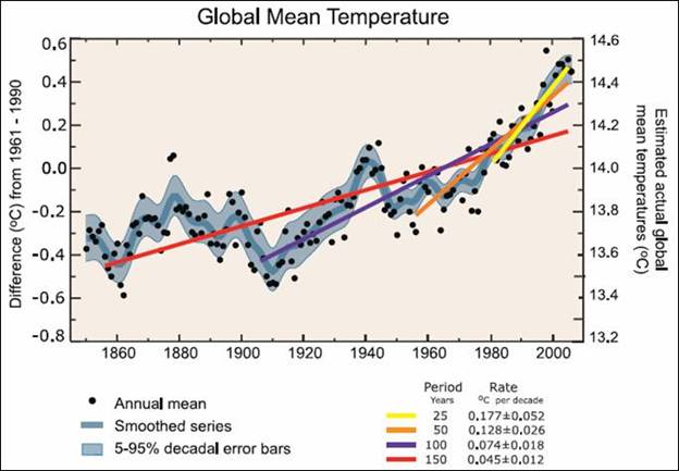
The UN IPCC AR4 states “Note that for shorter recent periods, the slope is greater, indicating accelerated warming.” But they create artificial acceleration by calculating short term linear trends within cyclical data. The following figure is Fig. FAQ 3.1 from Chapter 3 of the IPCC AR4 2007 report [http://www.ipcc.ch/pdf/assessment-report/ar4/wg1/ar4-wg1-chapter3.pdf]
What they are obfuscating is the cyclical variation in the actual data. The calculation of linear trends with disregard to the non-linear cyclical nature gives erroneous (or dishonest) results.
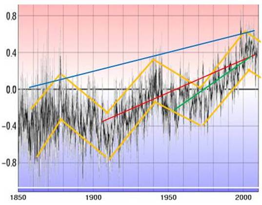
The following figure shows the HadCRU global temperature anomaly data that went into developing the above graph, along with orange lines indicating the 60-year cycle. The red line on the figure below shows the 0.74 degrees per century (shown in purple above), while the green line shows the 1.28 degrees per century (shown in orange above). Arbitrary linear trends within cyclical data will produce whatever the desired result is by choosing the start point appropriately.
The linear warming trend observed when accounting for the cycle is actually about 0.3 degrees per century as shown by the blue line on the figure below based on the trend in the peaks of the approximately 60-year cycle. And it has not been accelerating.
|
|
Food and Agriculture Organization – Fisheries Data
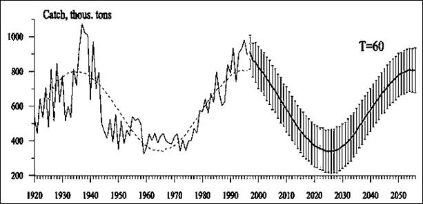
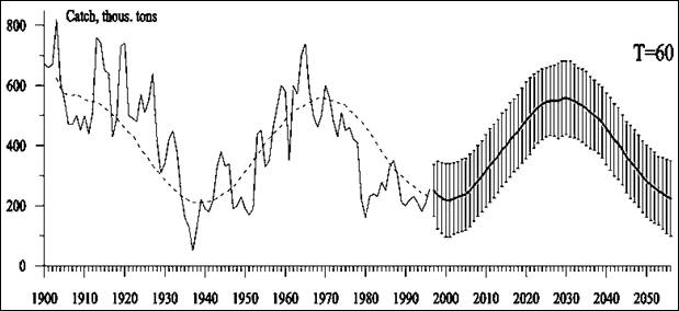
The UN FAO published a report in 2001 called “Climate change and long-term fluctuations of commercial catches” [ftp://ftp.fao.org/docrep/fao/005/y2787e/y2787e00.pdf]. The surprising thing about this report: they examined climate change in terms of the observed cyclical nature instead of assuming CO2 would drive everything to extinction (i.e. climate change in this case is not a euphemism for anthropogenic global warming). They also developed predictive models based on the observed cycles. The cycles were stated to have a period of somewhere between 55 – 65 years.
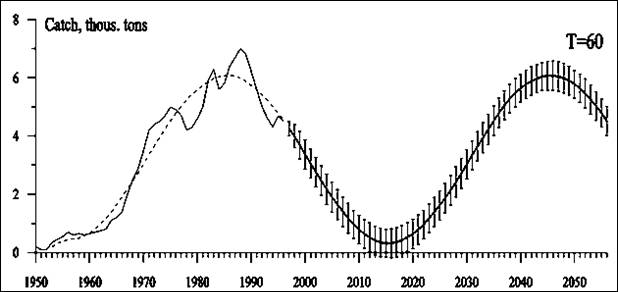
The following figures show some of the fishery models from the report.
Pacific Salmon Catch
Alaskan Pollock Catch
Pacific Herring Catch
From the FAO study:
The study found the Atmospheric Circulation Index (ACI) to be useful in determining climatic regimes. The ACI, developed by Russian climatologist George Vangengeim “Characterizes the periods of relative dominance of either "zonal" or "meridional" transport of the air masses on the hemispheric scale. … Meridional (C) circulation dominated in 1890-1920 and 1950-1980. The combined, "zonal" (W+E) circulation epochs dominated in 1920-1950 and 1980-1990. Current "latitudinal"(WE) epoch of 1970-1990s is not completed yet, but it is coming into its final stage … It was found that "zonal" epochs correspond to the periods of global warming and the meridional ones correspond to the periods of global cooling.”
One of the scientists involved in these studies was Leonid Klyashtorin who published a study comparing fish catches to climatic phenomena. He states: “This contradicts the conventional belief in “global warming”” [http://www.pices.int/publications/pices_press/volume5_issue2/May97/Pacific_Salmon.PDF]
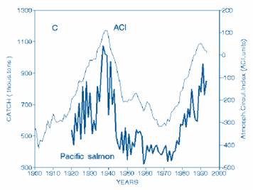
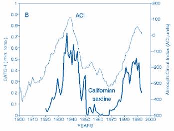
The following figures comparing fish catch to ACI are from Klyashtorin’s report.
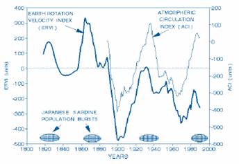
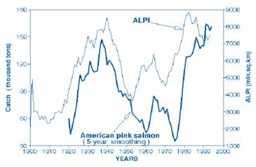
The following figures are also from Klyashtorin’s report, comparing ACI with Earth Rotational Velocity Index (ERVI) and comparing pink salmon catch with Aleutian Low Pressure Index (ALPI).
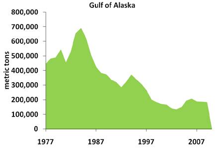
I tried to find fish catch data that could be compared to the FAO prediction graphs and found a graph for Alaskan Pollock as shown below. [http://www.nmfs.noaa.gov/fishwatch/species/walleye_pollock.htm]
The following figure compares the above to the FAO prediction shown previously.
|
|
The 60-Year Cycle
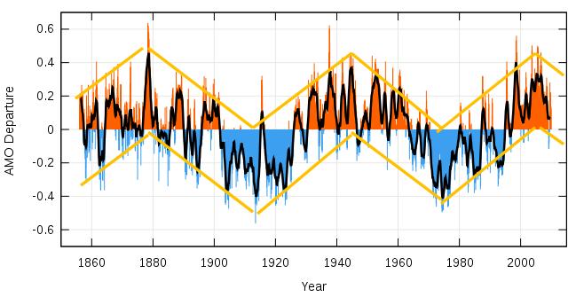
The climate cycle of approximately 60-year period is observable in many climatic phenomena. The following figure shows the Atlantic Multidecadal Oscillation (AMO) anomalies from 1850 to 2009 [http://en.wikipedia.org/wiki/File:Amo_timeseries_1856-present.svg].
The cycle length is approximately 62 years with maxima around 1878, 1943 and 2004, and minima around 1912 and 1974.
For an examination of various climate phenomena exhibiting the cycle (ENSO, PDO, US drought, etc.) see: http://www.appinsys.com/GlobalWarming/SixtyYearCycle.htm
|
|
|