Global Warming Science - www.appinsys.com/GlobalWarming
Climate Regime Shifts
[last update: 2010/08/03 – connections to solar magnetic phenomena updated]
|
“The notion that climate variations often occur in the form of ‘‘regimes’’ began to become appreciated in the 1990s. This paradigm was inspired in large part by the rapid change of the North Pacific climate around 1977 [e.g., Kerr, 1992] and the identification of other abrupt shifts in association with the Pacific Decadal Oscillation (PDO) [Mantua et al., 1997].” [http://www.beringclimate.noaa.gov/regimes/Regime_shift_algorithm.pdf]
|
|
Pacific Regime Shifts
Hare and Mantua, 2000 (“Empirical evidence for North Pacific regime shifts in 1977 and 1989”): “It is now widely accepted that a climatic regime shift transpired in the North Pacific Ocean in the winter of 1976–77. This regime shift has had far reaching consequences for the large marine ecosystems of the North Pacific. Despite the strength and scope of the changes initiated by the shift, it was 10–15 years before it was fully recognized. Subsequent research has suggested that this event was not unique in the historical record but merely the latest in a succession of climatic regime shifts. In this study, we assembled 100 environmental time series, 31 climatic and 69 biological, to determine if there is evidence for common regime signals in the 1965–1997 period of record. Our analysis reproduces previously documented features of the 1977 regime shift, and identifies a further shift in 1989 in some components of the North Pacific ecosystem. The 1989 changes were neither as pervasive as the 1977 changes nor did they signal a simple return to pre-1977 conditions.” [http://www.sciencedirect.com/science?_ob=ArticleURL&_udi=B6V7B-41FTS3S-2…]
Overland et al “North Pacific regime shifts: Definitions, issues and recent transitions” [http://www.pmel.noaa.gov/foci/publications/2008/overN667.pdf]: “climate variables for the North Pacific display shifts near 1977, 1989 and 1998.”
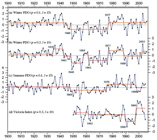
The following figure from the above paper show analysis of PDO and Victoria Index using the Rodionov regime detection algorithm. A regime shift is also detected around 1947-48.
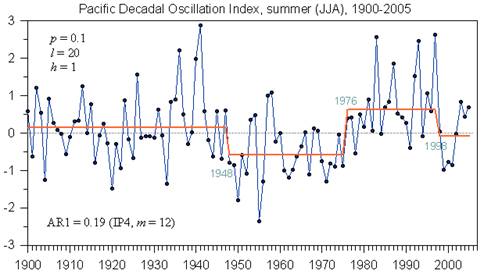
The following figure shows regime shift detection for the summer PDO, showing shifts at 1948, 1976 and 1998. [http://www.beringclimate.noaa.gov/data/Images/PDOs_FigRegime.html]
(For detailed information on the 1976/77 climate shift, see: http://www.appinsys.com/GlobalWarming/The1976-78ClimateShift.htm)
|
|
Regime Shift Detection in Annual Temperature Anomaly Data
The NOAA Bering Climate web site provides the algorithm for regime shift detection developed by Sergei Rodionov [http://www.beringclimate.noaa.gov/regimes/index.html]. The following analyses use the Excel VBA regime change algorithm version 3.2 from this web site.
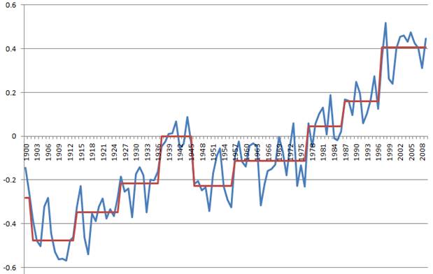
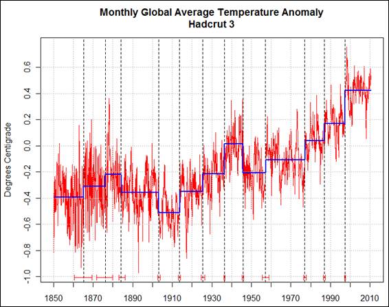
The following figure shows the regime analysis of the HadCRUT3 annual global annual average temperature anomaly data from the Met Office Hadley Centre for 1895 to 2009 [http://hadobs.metoffice.com/hadcrut3/diagnostics/global/nh+sh/annual].
The analysis was run based on the mean using a significance level of 0.1, cut-off length of 10 and Huber weight parameter of 2 using red noise IP4 subsample size 6. Regime changes are identified in 1902, 1914, 1926, 1937, 1946, 1957, 1977, 1987, and 1997. Running the analysis based on the variance rather than the mean results in regime changes in the bold years listed above.
|
|
Regime Shift Relationship to Solar Cycle
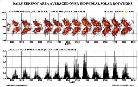
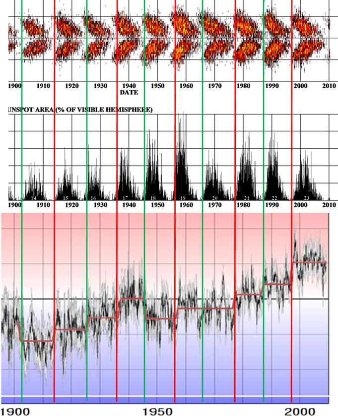
The NASA Solar Physics web site provides the following figure showing sunspot area. [http://solarscience.msfc.nasa.gov/SunspotCycle.shtml]
The following figure compares the Hadley (HadCrut3) monthly global average temperature (from [http://hadobs.metoffice.com/hadcrut3/diagnostics/global/nh+sh/]) overlaid with the regime change line (red line) shown previously, along with the sunspot area since 1900. The sunspot cycle is approximately 11 years. The sun’s magnetic field reverses with each sunspot cycle and thus after two sunspot cycles the magnetic field has completed a cycle – a Hale Cycle – and is back to where it started. Thus a complete magnetic sunspot cycle is approximately 22 years. The figure marks the onset of odd-numbered cycles with a vertical red line, even-numbered cycles with a green line.
From the figure above it can be seen that the regime changes correspond to the onset of solar cycles and occur when the “butterfly” is at its widest. The most significant warming regime shifts occur at the start of odd-numbered cycles (1937, 1957, 1977, 1997). Each odd-numbered cycle (red lines above) has resulted in a temperature-increase regime shift. Even-numbered cycles (green lines above) have been inconsistent, with some resulting in temperature-decrease regime shifts (1902, 1946) or minor temperature-increase shifts (1926, 1987).
An unusual one is the 1957 – 1966 cycle, which in the monthly data shown above visually looks like a temperature-increase shift in 1957 followed by a temperature-decrease shift in 1964 but the regime detection algorithm did not identify it. This is likely due to the use of annually averaged data in the regime detection algorithm.
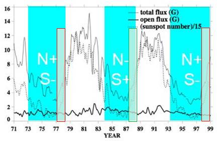
The following figure shows the relative polarity of the Sun’s magnetic poles for recent sunspot cycles along with the solar magnetic flux [www.bu.edu/csp/nas/IHY_MagField.ppt]. The regime change periods are highlighted by the red and green boxes. Each one occurs on as the solar cycle is accelerating. The onset of an odd-numbered sunspot cycle (1977-78, 1997-98) occurs during the relative alignment of the Earth’s and the Sun’s magnetic fields (positive North pole on the Sun) allowing greater penetration of the geomagnetic storms into the Earth’s atmosphere. “Twenty times more solar particles cross the Earth’s leaky magnetic shield when the sun’s magnetic field is aligned with that of the Earth compared to when the two magnetic fields are oppositely directed” [http://www.nasa.gov/mission_pages/themis/news/themis_leaky_shield.html]
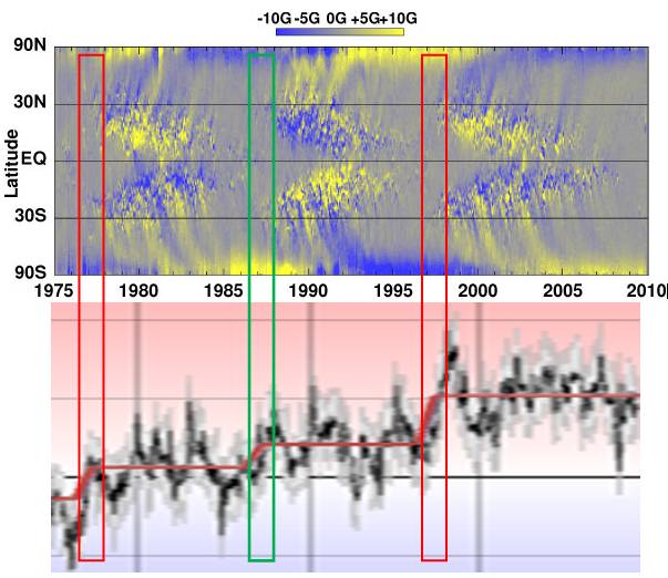
The following figure shows the longitudinally averaged solar magnetic field. This “magnetic butterfly diagram” shows that the sunspots are involved with transporting the field in its reversal. The Earth’s temperature regime shifts are indicated with the superimposed boxes – red on odd numbered solar cycles, green on even. [http://solarphysics.livingreviews.org/open?pubNo=lrsp-2010-1&page=articlesu8.html]
The Earth’s temperature regime shift occurs as the solar magnetic field begins its reversal.
|
|
Solar Cycle 24
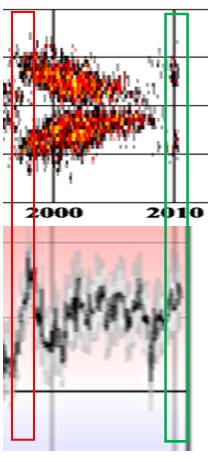
Solar cycle 24 is in its initial stage after getting off to a late start. An El Nino occurred in the first part of 2010. This may be the start of the next regime shift.
|
|
Comparison With Other Analysis Methods
There has been considerable discussion on this page at Watts Up With That (see: http://wattsupwiththat.com/2010/07/05/spotting-the-solar-regime-shifts-driving-earths-climate/)
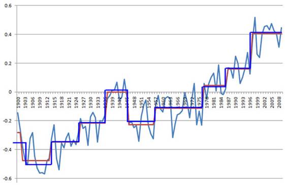
A commenter on that forum – Rich – used the R package “strucchange” function to perform a similar analysis on the HadCrut3 monthly data. His results are shown below (monthly anomaly data in red). Confidence interval bars for each regime shift are plotted in red near the x-axis.
Rich’s regime shifts from above, based on monthly data, are shown below (blue line) compared with the previous regime shift algorithm results (red line) which were based on the annual data.
|
|
Solar Geomagnetic Ap Index
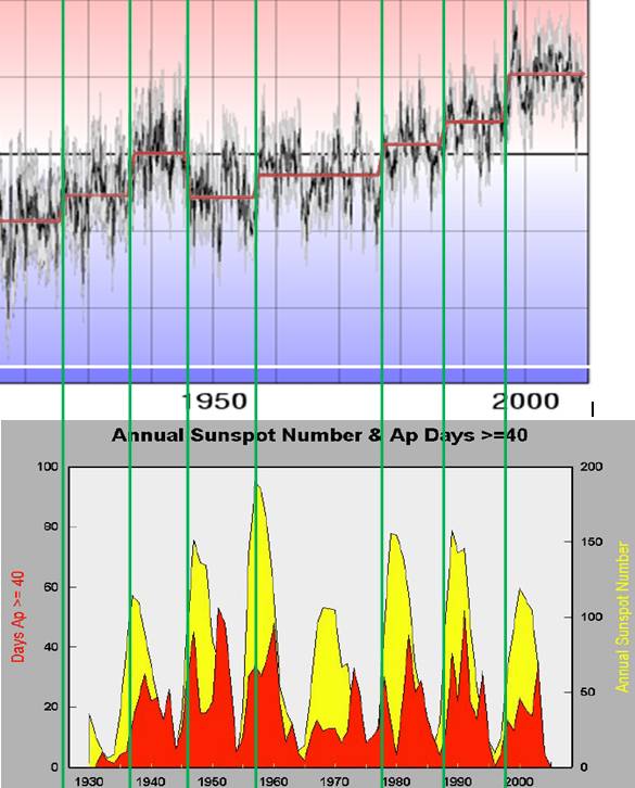
The Ap Index was introduced in 1975. “It is computed as the 8-point running average of successive 3-hourly ap magnetic activity indices. When the average rises above an arbitrary threshold (usually 40), a major magnetic storm is considered to be in progress. While the running average stays above the threshold, it is considered one storm.” [http://www.scostep.ucar.edu/archives/scostep11_lectures/Allen.pdf] The following figure compares the identified regime shifts to the Ap Days >= 40 (red) from that report. Again they correspond to the ramping up from a minimum.
|
|
Coincidence With Geomagnetic Storms based on Kp
The Kp index was introduced in 1949 based on the disturbance levels in the horizontal magnetic field components and subsequently extended back to 1932 [http://www-app3.gfz-potsdam.de/kp_index/description.html].
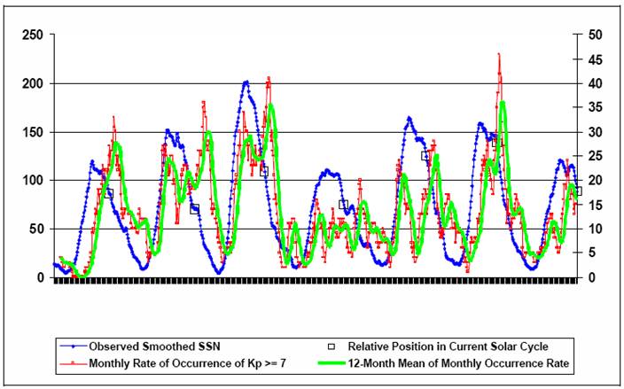
The following figure shows the monthly rate of occurrence of severe geomagnetic storms (i.e. with Kp > 7) (red) and the 12-month moving average of the same (green), along with sun spot number (blue) [http://www.spacew.com/gic/guidance.pdf]
The following figure combines the above graph with the graph shown previously.
An interesting coincidence: the temperature regime shifts occur when the decreasing geomagnetic storm rate crosses the increasing sun spot number.
The only solar cycle without an identified regime shift at its onset is solar cycle 20, starting in 1966. It is coincidental that the decreasing geomagnetic storm rate occurs earlier than usual and it makes a double dip. This is highlighted by the blue circle above.
|
|
Geomagnetic aa Index
The aa index is based on 3-hour antipodal geomagnetic observations in Britain in the Northern Hemisphere and locations in Australia in the Southern Hemisphere.
Cliver et al (“Solar variability and climate change: Geomagnetic aa index and global surface temperature”, Geophysical Research Letters, Vol.25, 1998) state: “During the past ∼120 years, Earth's surface temperature is correlated with both decadal averages and solar cycle minimum values of the geomagnetic aa index. The correlation with aa minimum values suggests the existence of a long‐term (low‐frequency) component of solar irradiance that underlies the 11‐year cyclic component. … the general similarity in the time‐variation of Earth's surface temperature and the low‐frequency or secular component of the aa index over the last ∼120 years supports other studies that indicate a more significant role for solar variability in climate change on decadal and century time‐scales than has previously been supposed.” [http://www.agu.org/pubs/crossref/1998/98GL00499.shtml]
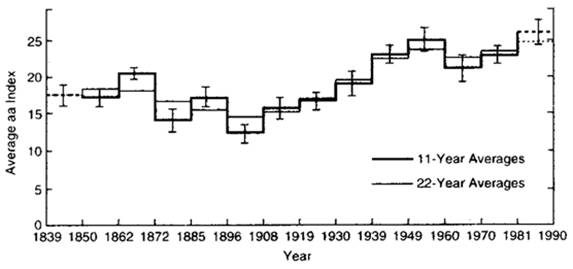
The following figure shows “the "11-year" solar cycle average of the aa index beginning two years after solar maximum (heavy line), together with the double solar cycle average which removes the "22-year" periodicity.” (From Russell and Mulligan “The 22-year Variation of Geomagnetic Activity: Implications for the Polar Magnetic Field of the Sun”, 1995 [http://www-ssc.igpp.ucla.edu/personnel/russell/papers/731/731index.htm])
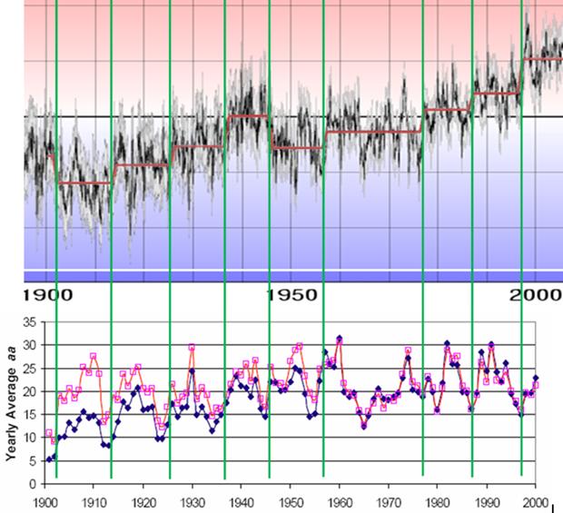
The following figure shows the above average aa index lines changed to green and superimposed on the regime changes identified by Rich using R-strucchange (blue) and the monthly HadCRUT3 anomaly data (red). The regimes are out of sync with the averages since the averages were based on starting “two years after solar maximum”. The aa 11-year averages have a good correspondence to the temperature trends and shifts.
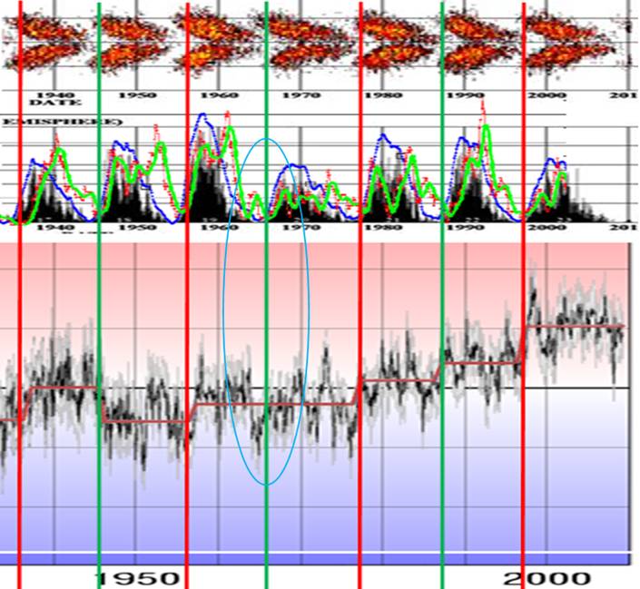
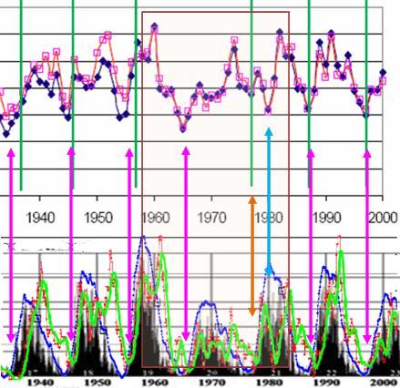
Leif Svalgaard et al developed “a new simplified daily index of geomagnetic activity [IHV] that is well suited for studies of the long-term variability of solar-terrestrial interactions.” [http://www.leif.org/research/IHV%20-%20a%20new%20long-term%20geomagnetic%20index.pdf] The following figure compares the regime shifts identified previously with the geomagnetic aa index from the Svalgaard paper (aa index in dark blue, aa index reconstructed from IHV in pink).
The above shows a strong correspondence between the regime shifts and the start of the rise of the aa index from each minimum. The exception is the 1965 minimum and the 1977 shift leads the 1980 minimum. This 1960-1980 timeframe is highlighted below comparing it to the Kp > 7 rate shown previously. The early 1960s – late 1970s was an unusual solar cycle in terms of Kp storms. The magenta arrows indicate the typical coincidence of the aa index minimum with the crossing of the sunspot / Kp7 storm lines. The aa index / Kp7 storm crossing get out of sync in the 1970s, although the 1977 regime shift matches the Kp7-SSN crossing. This indicates that the Kp7 is more correlated to the climate regime shifts than the aa index.
|
|
Temperature Analysis using Hodrick-Prescott Filtering
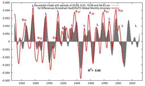
In 2009 Basil Copeland and Anthony Watts did an analysis involving a Hodrick-Prescott filter on the monthly HadCRUT anomaly data [http://wattsupwiththat.com/2009/05/23/evidence-of-a-lunisolar-influence-on-decadal-and-bidecadal-oscillations-in-globally-averaged-temperature-trends/] The following figure is from that analysis, showing the first differences of trend component smoothed (red line) as well as the result of a sinusoidal model (gray).
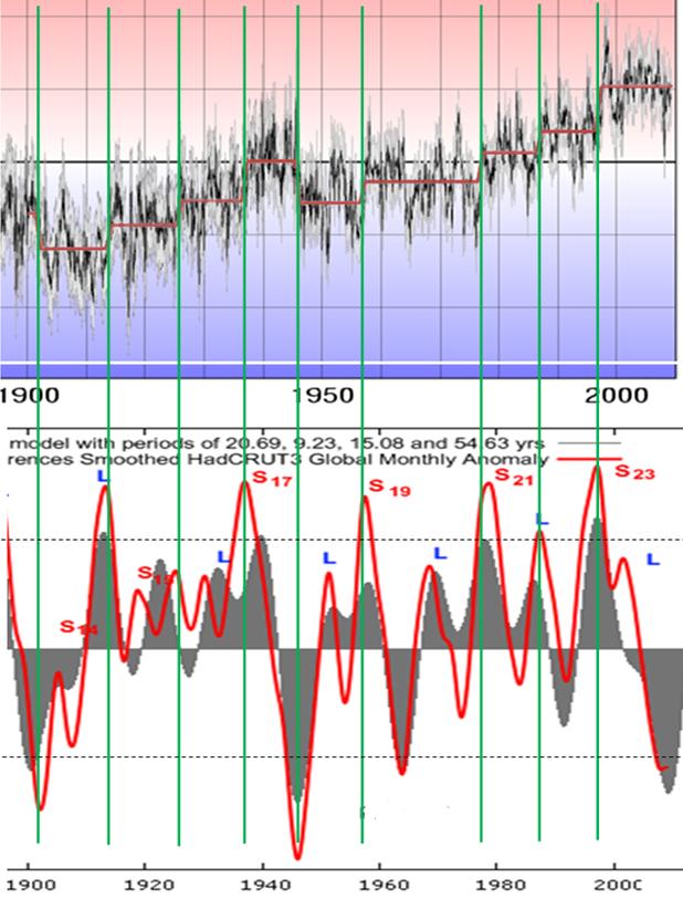
The following figure compares the regime shifts identified previously with the first differences smoother (red) line from the above graph.
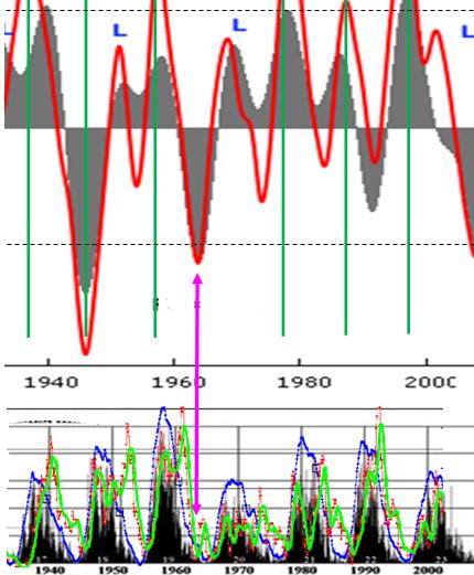
The regime shifts occur whenever the first difference curve is > +/-0.0025 (indicated by the dotted lines on the lower graph above). There are two exceptions: 1) a regime shift was identified in 1926 when the first difference curve has low oscillations not reaching the 0.0025 level; 2) no regime shift was identified in 1963 when the first difference line slightly crossed the -0.0025 level. The 1964 temperature drop corresponded to an unusual drop in the rate of Kp > 7 as shown below.
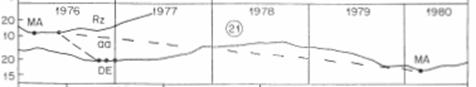
Sunspot cycle 21 was unusual: “A very unusual thing occurred in cycle 21 when aa had two minima, one in November 1976 (five months after the Rz(min) of June 1976), and another several years later, in March 1980.” [http://hal.archives-ouvertes.fr/docs/00/31/71/67/PDF/angeo-20-1519-2002.pdf] The following figure is from that paper showing the initial aa index minimum (DE in 1976) corresponding to the regime shift and orange arrow above, and the later lower minimum (MA in 1980) as indicated by the blue arrow above.
The evidence indicates that the climate regime shifts identified correspond to the interaction of decreasing geomagnetic storms (Kp > 7) with increasing sunspot area.
|
|
|